The "Apply formulae by key" action step is a powerful tool for large spreadsheets that contain a lot of formulas. This step applies a formula to a cell, depending on the value of another cell in the same row (the key). The power and great use of this step can be easily seen when applying to large datasets with a large number of rows, each with varying formulas for each column.

One large benefit of this step is it allows you to avoid having to use messy and confusing "IF" statements in Excel that are usually quite difficult to debug or understand when these statements contain complicated formulas or when multiple "IF" statements are nested.

To best highlight the use of this step, we will go through an example that will use this step.

Note: this step only uses the leftmost cell in each row as the "key".

Example

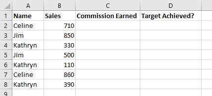
In this example, we have a dataset containing a list of sales representatives with their respective sales amounts for the month.

Furthermore, each sales representative has their own target sales threshold. If they make a sale above this threshold, they receive a prize. 

We wish to work out the amount of commission that each person has earned, as well as whether they have reached this threshold.

Below is a screenshot of the sample data (stored in a tab called "Data"):

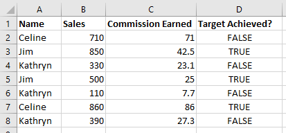
However, suppose that Jim earns a 5% commission rate, Kathryn earns a 7% commission rate and Celine earns a 10% commission rate.

Furthermore, Jim's target sales is $400, Kathryn's target sales is $600 and Celine's target sales is $800.

This information can be summarised by the following formula template (stored in a separate tab called "Formula Template":

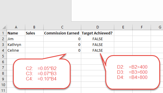
That is, column C will apply the appropriate commission rate to column B, given the name in column A for the same row.

Similarly, column D will apply the appropriate check to column B, given the name in column A for the same row.

For example, for every row in the "Data" tab, each row that has "Kathryn" in column A will calculate column C as 7% of the value in column B.

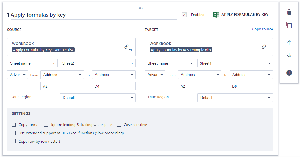
Creating the step

We now have enough to use the "Apply formulae by key" step.

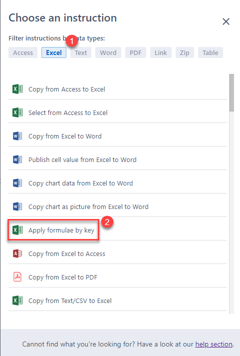
Firstly, create an action step to manipulate data and select "Apply formulae by key" in the "Excel" section.

Next, you will see the following 

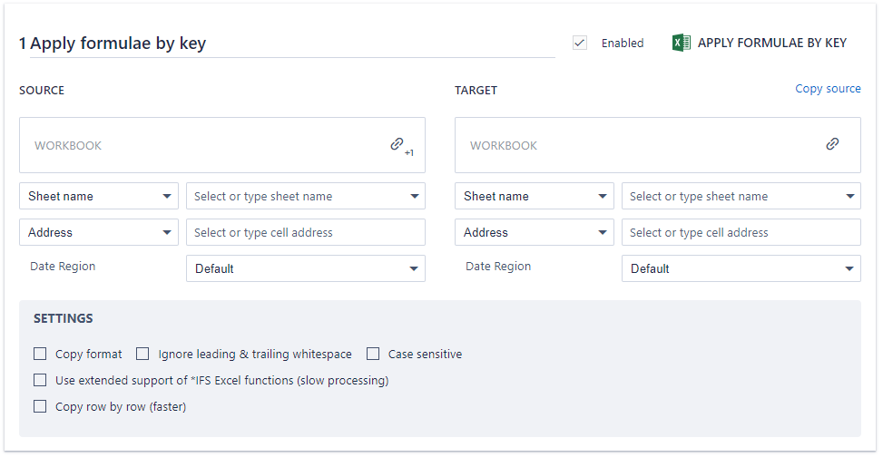
There are two main parts to this step:

- configuring the source range (where the template formulas are)

- configuring the target range (the data that we wish to apply the formulas on)

In our example, the source range, which contains the formulas will be in the range A2 to D4.

The target range, which contains the data is the range A2 to D8.

The completed instruction is given below.

Once the step is run, the final output will automatically apply the correct formulas based on the formula template and provide the following output.

Note: the optional checkboxes at the bottom allow for more flexible use, such as the ability to apply the formatting of the cell as well as the formulas, or the ability to ignore leading and trailing whitespace or the restriction of case sensitivity.