The Copy pivot table instruction, in conjunction with the Refresh pivot tables instruction, is necessary to process Excel files which contain pivot tables.

Very often, processes in SolveXia are designed to populate the Excel file with the latest data. This data is then fed into pivot tables.

Later in this article, we will go through one such example to illustrate how this instruction can be used to maintain pivot tables in Excel files through SolveXia.

How to use this instruction to maintain pivot tables

1. Upload the relevant Excel workbook into a data step property. Ensure that the copy that is uploaded still contains the pivot table and is configured correctly.

2. Use the Copy Step Properties between Steps action to create a working file copy of this template. (There should now be two copies of the same file)

3. Run all Excel calculation instructions in the process on the working file copy. 

4. At the end of the process, add a Copy Pivot Table instruction to copy over the original pivot table in the template file back into the working file copy and then add a "Refresh Pivot Table" instruction to populate the pivot table with the new data.

Note: the original pivot table should already be pre-configured to the desired pivot table structure, such as values to display and source data range.

Note 2: the "Copy pivot table" and "Refresh pivot tables" instructions MUST only be after all other Excel calculations steps for the pivot table to be correctly maintained.

Example

In this example, the process has been designed to allow the end-user to upload the latest quarter's data into SolveXia, which will then generate a report containing a pivot table.

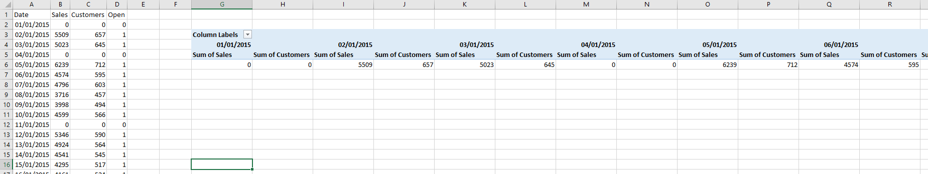
The dataset used involves sales data for a pharmacy in the 1st quarter of 2015.

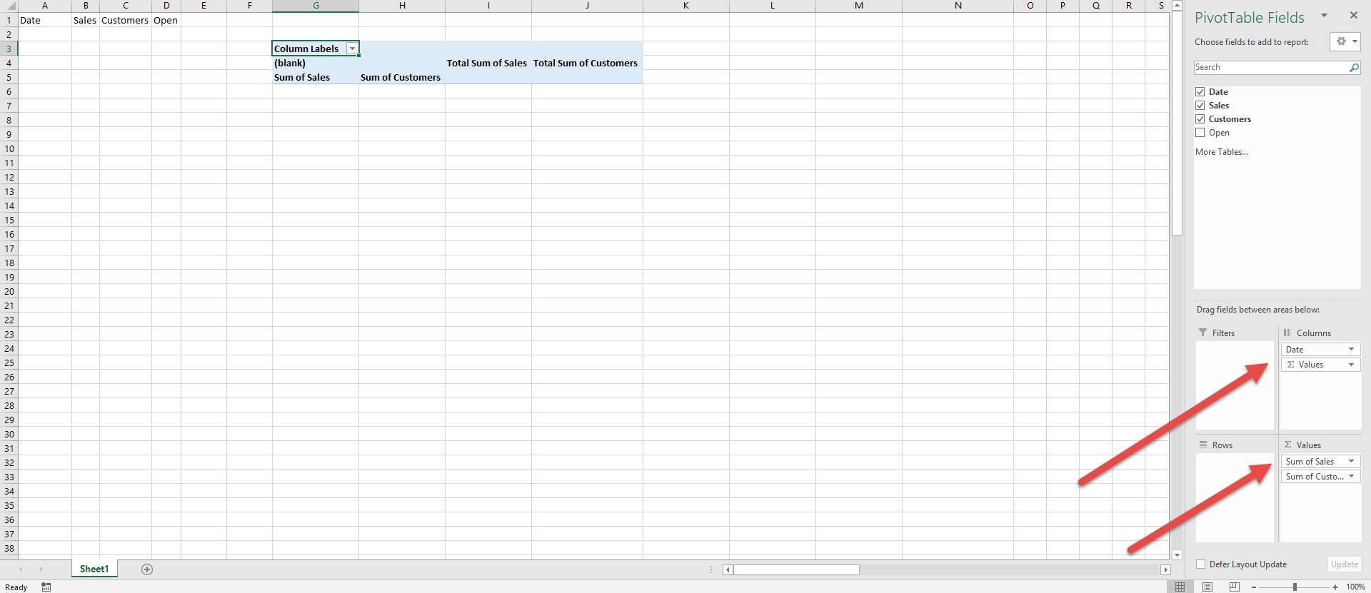The template file should contain the pivot table, pre-configured with the desired values to display as well as the source data range.

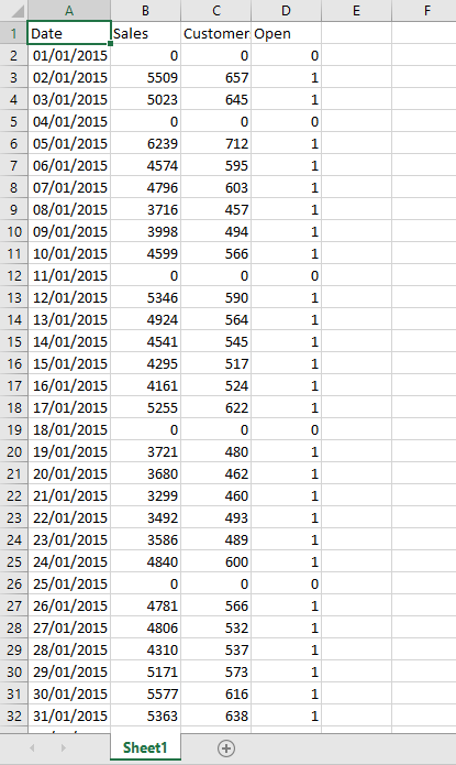
Here, the process will copy over the uploaded data for the 1st quarter of 2015 into columns A to D. 

And so, the data source range of the pivot table has been pre-emptively set to columns A to D in the template file.

Setting up the data step properties

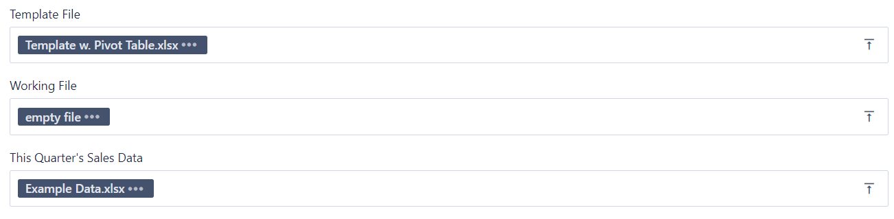
Firstly, we need to create three data step properties to hold:

• the template file
• the working file
• the uploaded data file

Creating a working file copy

Next, we need to create a working file copy of the template file. This file will be where the data is copied to and run through the Excel calculations steps in the rest of the process.

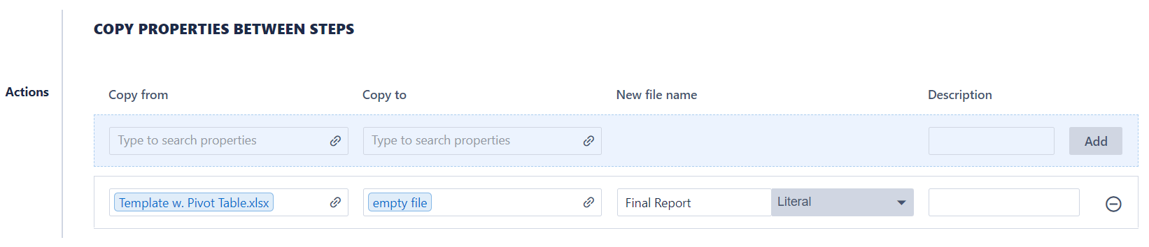
This can be done with a Copy step properties step, as configured above.

Once this step has been run, an exact copy of the template can be found in the "Working File" data step property called "Final Report.xlsx".

Running Excel calculation steps on the file

Once this is done, you can add all the relevant Excel-related instructions intended for this file.

In this simple example, we will only need to use the "Copy cell values" instructions to copy over this quarter's data. 

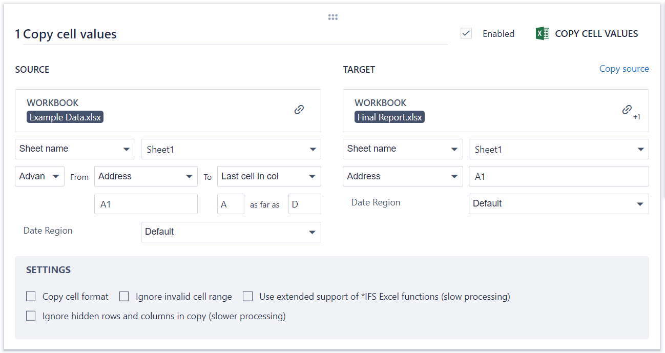
However, theoretically, here you can add all necessary Excel instructions required to generate the desired output, before dealing with the pivot tables.

Using the Copy pivot table instruction

Once all the calculations steps have been run in the Excel file, the last thing to do is to copy over the pivot table into the working file copy, to generate the final output.

This instruction simply copies over the pivot table "structure", in that the data source range and pivoted columns and rows are preserved.

And so, you will need to create a new action step to Manipulate Data and select the Copy pivot table instruction: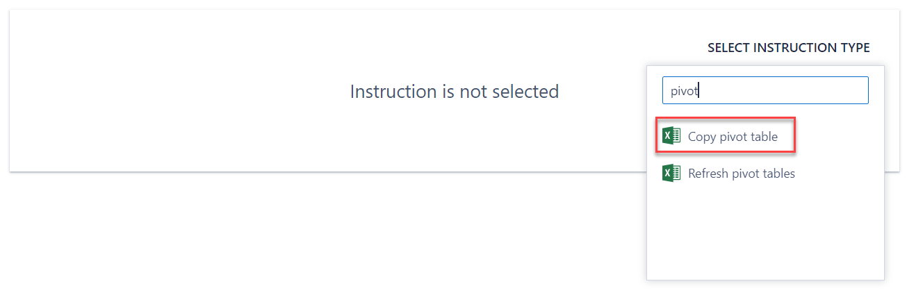

This instruction can then be configured as shown below:

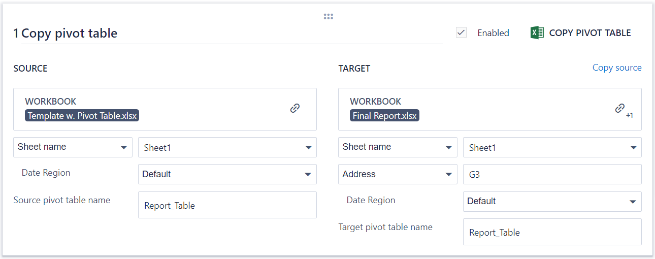
Note that the source workbook will be the template file. This file should not have been touched by any of the action steps done previously in the process (i.e. will not contain the uploaded data). All action steps should have been dealing with the working file copy.

The target workbook will be the working file. This file will now contain the uploaded data.

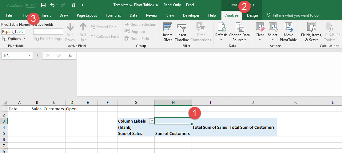
Note: To find the name of the source pivot table, simply click on any cell in the pivot table, then click on "Analyze" at the top ribbon in Excel and the name will appear in the "PivotTable Name" section on the left.

Once this is done, your pivot table should now successfully appear in the final output workbook.

Note: the pivot table will still not update to the new data set, as the pivot table will still need to be refreshed or "updated". You will now need to use the "Refresh pivot tables" instruction to finally populate the latest data into the final output workbook.

Tips & tricks

If a pivot table is configured to have a data source range for an entire column, then any blank rows will also be fed into the pivot tables and create an unnecessary pivot. 

However, more often than not, the number of rows in the data source is not known in advance, since the number of rows changes as more data is added or removed.

And so, to avoid including such blank rows in the source data range, we can use a dynamic named range to include all the rows up to the last filled-in row to circumvent this problem.

For more details, please refer to the Create named range article and use the "Last Cell in Col" feature to create a dynamic named range.